Building simple AOCS hardware in the loop test setup
This article provides short summary of achievements during 3 months internship at N7 Space held during summer 2026.
Motivation
We wanted to check how control algorithms behave on the target processor rather than only on a PC. For that purpose, we built a simulation, connected it to an actual onboard computer, and fed the simulation data to hardware, to measure things like computing time and memory use.
We built the scenario in Basilisk, an open-source astrodynamics framework with visualization in Vizard. It provides orbital mechanics, attitude dynamics, reaction wheel and thruster models.
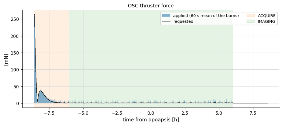
The AOCS (Attitude and Orbit Control System) is the part of the spacecraft software that keeps it pointing and positioned where it should be; in our case it uses reaction wheels to point each spacecraft at the Sun or at its partner, and thrusters to hold their relative position in the formation.
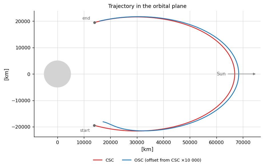
The scenario is inspired by the PROBA-3 mission: two spacecraft flying in formation, with the pointing targets being the Sun and the other spacecraft. Formation flight is a useful test case because attitude and position are controlled at the same time, for two vehicles, and the relevant behaviour is in how they hold relative to each other.
Every step the simulation produces, for both spacecraft: position, velocity, attitude as Modified Rodrigues Parameters (MRP), angular rates, reaction wheel speeds and the current pointing target. That is 37 values in total, including a timestamp.
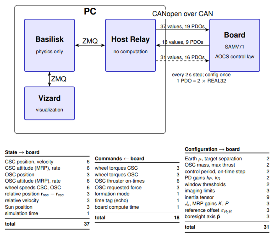
From that the controller computes the reference attitude and the attitude and rate error against it, the commanded torque from a proportional-derivative control law, mapped onto the reaction wheels, the force needed to hold the relative position, converted into thruster on-times. Which come back as 17 values.
The objective was to obtain results comparable to the software-only run, with the control math moved onto the board.
Hardware-in-the-Loop setup
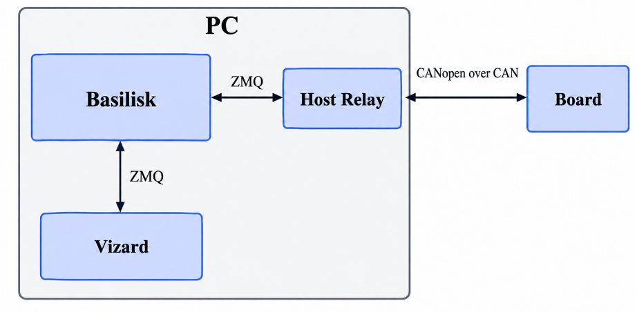
Software executed by OBCU (Onboard Computing Unit) is looped and it feeds values as if they came from a real satellite. It receives the simulated sensor data over the bus, computes the control commands, and sends them back the same way. From the board’s point of view the interface is the same one it would have on a spacecraft.
The host relay performs no computation. It reads values from the Basilisk’s ZMQ socket, parses them, writes them into CANopen objects, and passes the results back to the simulation. It serves only as a way of integrating Basilisk with real hardware.
The loop runs in lockstep, so the simulation waits for the board’s response before advancing. This makes runs repeatable, which is useful for a tests and benchmarks.
CANopen
CANopen was selected for communication between the board and the PC. Since it is the protocol used on board, the test runs on the actual interface, with the same framing and transmission format as in flight.
We move 86 values in total: 37 to the board each cycle, 17 back, and 31 configuration values at startup. Both the relay on the PC and the firmware on the board must interpret each of these values the same way, meaning they must use the same address, data type and position within a message. Otherwise, one side would send a value and the other would read it as something else. CANopen describes all of this in a so-called Object Dictionary, where every value has an address, a type and a fixed place in a message. We generate the code for both sides from the same DCF files (Device Configuration Files, a device-specific form of an EDS, Electronic Data Sheet), so they always match. If we wrote the two layouts by hand, they could differ without anyone noticing, and the data would still look valid.
CANopen PDO (Process Data Objects) service was used for control loop. A synchronizes Object Dictionary using small messages (single CAN frame) sent by the value producer. There is no request and no reply, so one update costs one message. We configure the mapping once, and after that the data is sent whenever it changes. This is a standard mode in CANopen, next to the synchronous mode, and the standard also limits how often one object can be sent, so a busy value cannot take over the bus. The protocol brings everything around the data as well: node addresses, the start-up state machine, heartbeats that show the board is alive, and error signaling. Configuring complete CANopen nodes required only preparing proper dictionary settings, library took over remaining setup.
On a board with 384 KiB of RAM this matters, because it means less space of our own code. The dictionary is machine-readable, so the code on both sides is generated. Any CANopen tool can also read the bus without knowing anything about our application.
Results
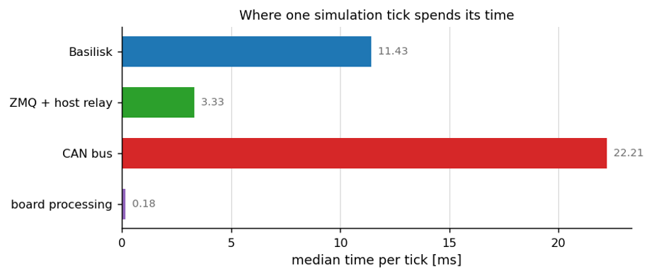
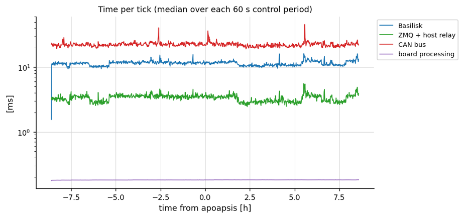
One full control cycle takes about 184 µs on average, measured on the board over 3804 cycles. The control loop runs once per simulation step, and one step is 2 s of simulated time (which comes from thrusters way of work – smaller time wouldn’t give modelled thrusters an opportunity to fire, that’s why we were simulated every 2 s, so in flight the board have 2 s to answer. It needs 150 µs of that, which is roughly one thirteen-thousandth. The same processor could run this loop 13 000 times per period and still finish on time. Which gives us room for a heavier or faster control loop.
The firmware uses 330 KiB of the 384 KiB of on-chip RAM, which leaves 54 KiB free. The memory usage could also be optimized, as it has big CANopen memory pool for possible extensions with other sensor data.
The biggest part is the object dictionary generated from the DCF. It grows with the number of values we exchange. The complexity of the control law does not change it. So adding math is cheap here, and adding telemetry fields is what costs.
Moving to the bus – control cycle carries 54 values, 37 in and 17 out. They are packed two per PDO, so 28 messages and 216 bytes per cycle. At 1 Mbit/s that is 3.1 ms of bus time per cycle, which is 0.16% of the 2 s period. The bus alone could carry about 320 full control cycles per second. On the test bench the cycles came much faster than that. The lockstep loop does not wait for the clock, it runs as fast as the link allows, so one cycle took 90 ms of real time, measured as the median over the run. Against that faster rate the board still used only 0.17% of each cycle and the bus 3.45%. The remaining 99.83% of those 90 ms was transport. This transport time comes from our test setup: the board is in another location and the CAN bus is tunnelled to it over the network
Conclusion
We can run a control algorithm on target hardware against realistic dynamics. The same setup can be used for other scenarios and other boards. Create simulation, algorithm, send data to hardware and there you get a result.
Reference
- PROBA-3
- Software used for simulation
- Basilisk
- CANopen library and ECSS Test Suite
- Manim